Mastering Lineplots_LB

In this vingette we will see how to master the Lineplots_LB function to build perfect lineplots. First we configure the environment and load all necessary packages.

options(scipen = 999999)
library(LandS)
library(ggplot2)

After that we can load the dataframe from which we will run the lineplots.

set.seed(2201)
data01 <- data.frame(ID = rep(paste0("PT-", 1:6), each = 5), 
                     Time = rep(1:5, 6), 
                     Marker_1 = rnorm(30), 
                     Marker_2 = rnorm(30, 0, 5), 
                     Marker_3 = rnorm(30, 0, 2), 
                     Gender = factor(rep(c("M", "F"), each = 5, length.out = 30), 
                                     levels = c("M", "F"), ordered = TRUE))

In this case the generated data is simulated, for more info on how to set a dataframe compliant with the LandS package consult the “Getting Started” vignette

Single graph

You can build a single graph using the following code:

Lineplots_LB(data = data01, 
             variables = "Marker_1", 
             time = "Time")
#> Loading required package: ggpubr
#> Loading required package: dplyr
#> 
#> Attaching package: 'dplyr'
#> The following objects are masked from 'package:stats':
#> 
#>     filter, lag
#> The following objects are masked from 'package:base':
#> 
#>     intersect, setdiff, setequal, union
#> Loading required package: ggh4x
#> Loading required package: grid
#> Loading required package: gridExtra
#> 
#> Attaching package: 'gridExtra'
#> The following object is masked from 'package:dplyr':
#> 
#>     combine
#> Loading required package: svMisc
#> 
#> Attaching package: 'svMisc'
#> The following object is masked from 'package:utils':
#> 
#>     ?
#> Loading required package: officer
#> Loading required package: rvg
#> Loading required package: progress
#> 
#> Attaching package: 'pryr'
#> The following object is masked from 'package:dplyr':
#> 
#>     where
#> ██████████████████████████████████████████████████████████████████████████████████████████ 100%  00:00:00 | ETA: 00:00:00 | RAM: 0.07Gb
#> [[1]]

You can see that the arguments used by the function are:

data, the dataframe
variable, the variable to build the lineplots
time, the x-axis variable

Customize a single graph

We can change the lineplot graphics as follows:


Lineplots_LB(data = data01, variables = "Marker_1", time = "Time")
#> ██████████████████████████████████████████████████████████████████████████████████████████ 100%  00:00:00 | ETA: 00:00:00 | RAM: 0.08Gb
#> [[1]]

Single graph split by a group variable

We can also get separated curves for a specific grouping variable:

Lineplots_LB(data = data01, variables = "Marker_1", time = "Time", group = "Gender")
#> ██████████████████████████████████████████████████████████████████████████████████████████ 100%  00:00:00 | ETA: 00:00:00 | RAM: 0.08Gb
#> [[1]]

Build a list of lineplots

Lineplots_LB(data = data01, variables = c("Marker_1", "Marker_2"), time = "Time", group = "Gender")
#> █████████████████████████████████████████████░░░░░░░░░░░░░░░░░░░░░░░░░░░░░░░░░░░░░░░░░░░░░  50%  00:00:00 | ETA: 00:00:00 | RAM: 0.08Gb██████████████████████████████████████████████████████████████████████████████████████████ 100%  00:00:00 | ETA: 00:00:00 | RAM: 0.08Gb
#> [[1]]

#> 
#> [[2]]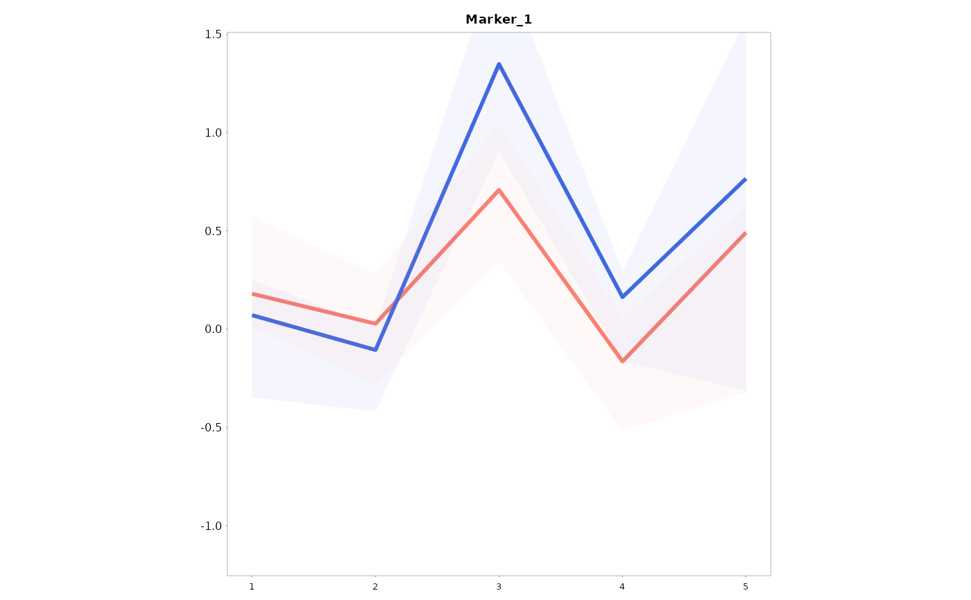

#> 
#> [[3]]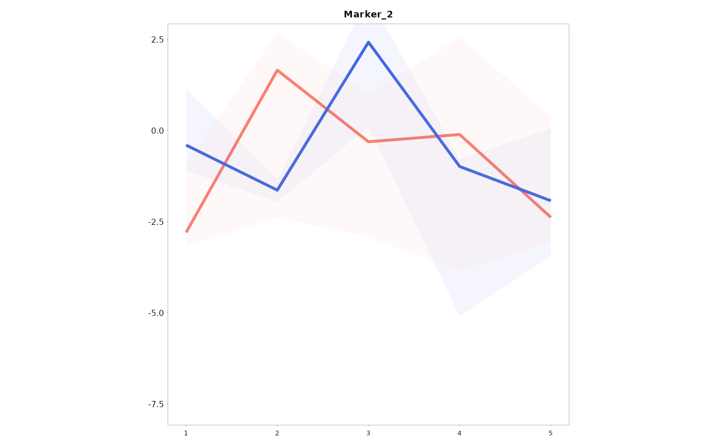

Save a list of lineplots

You can save a list of lineplots in two different ways: you can build a grid and save the entire grid in a pdf file, or you can generate a PPTX file with every lineplot in a different slide.

Save a list of lineplots as a pdf grid file


List_reg <- Lineplots_LB(data = data01, variables = c("Marker_1", "Marker_2"), time = "Time", group = "Gender")

LandS::Print_LB(plot_list = List_reg, path_print = "your/directory", ext = "pdf")

Save a list of lineplots as a PPTX file

Lineplots_LB(data = data01, variables = c("Marker_1", "Marker_2"), time = "Time", group = "Gender", 
             PPTX = TRUE, grid = FALSE, pptx_width = 6, pptx_height = 4, target = "your/directory/new_presentation.pptx")

Customize the colour of the title

library(dplyr)
df_legend <- matrix(ncol = 2, nrow = 2) %>% as.data.frame() %>% `colnames<-`(c("Var", "Colour"))
df_legend$Var <- c("Marker_1", "Marker_2")
df_legend$Colour <- c("red", "orange")

colour_title <- function(i) df_legend$Colour[df_legend$Var == i]

Lineplots_LB(data = data01, variables = c("Marker_1", "Marker_2"), time = "Time", group = "Gender", 
             col_title = TRUE, colour_title = colour_title)
#> █████████████████████████████████████████████░░░░░░░░░░░░░░░░░░░░░░░░░░░░░░░░░░░░░░░░░░░░░  50%  00:00:00 | ETA: 00:00:00 | RAM: 0.08Gb██████████████████████████████████████████████████████████████████████████████████████████ 100%  00:00:00 | ETA: 00:00:00 | RAM: 0.08Gb
#> [[1]]

#> 
#> [[2]]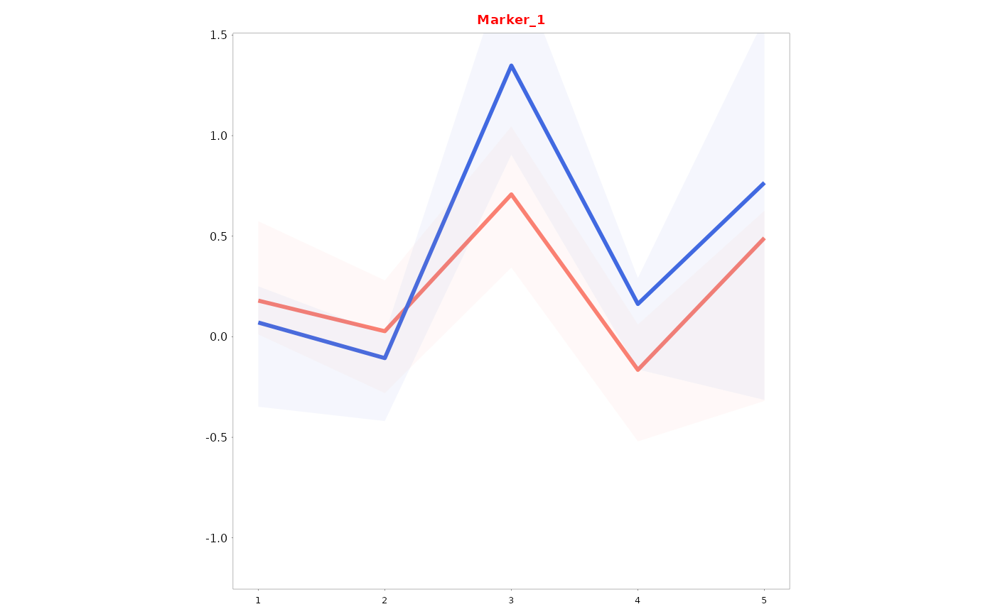

#> 
#> [[3]]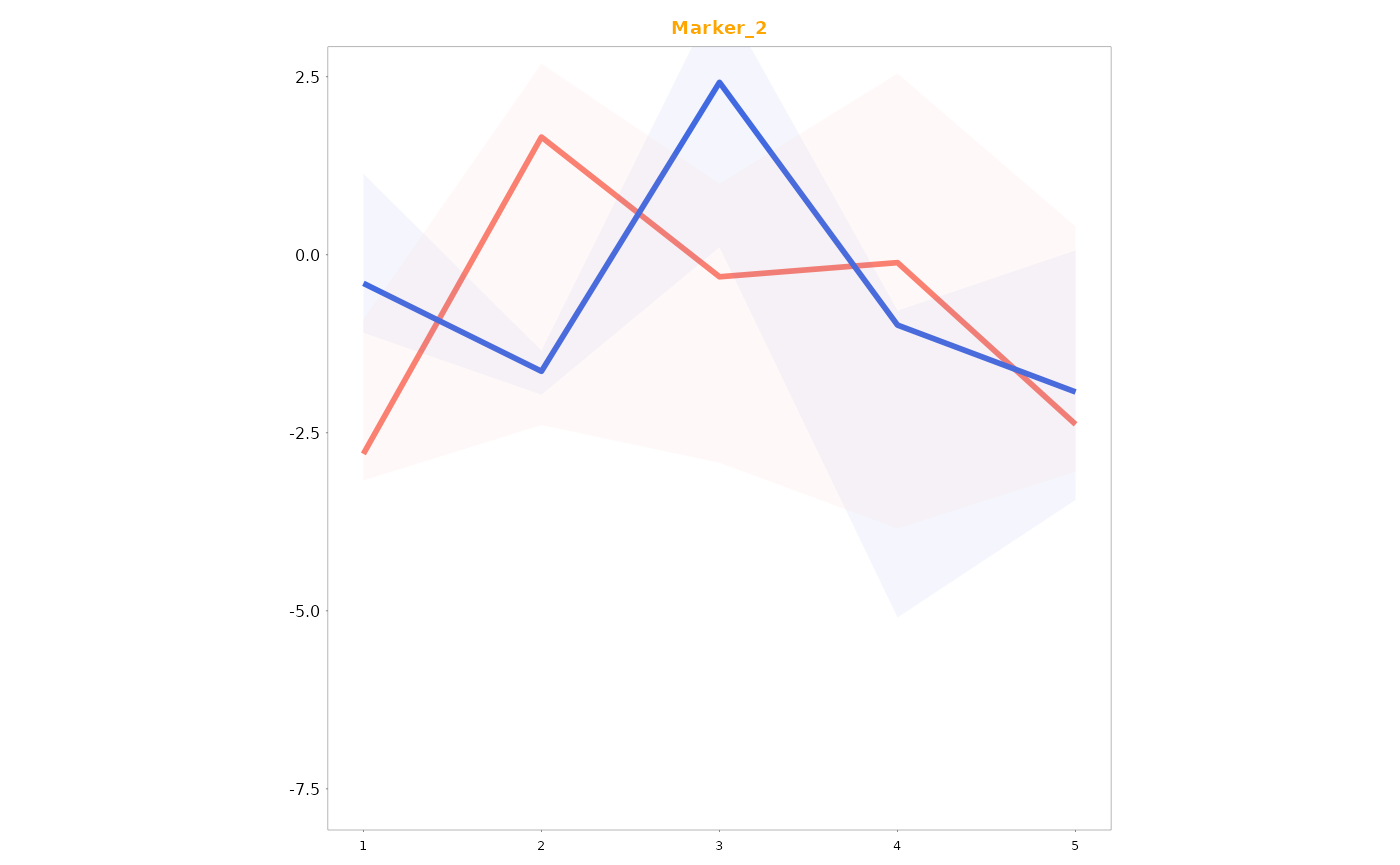

Add overall and posthoc tests to the graphs

# Let's make the grouping variable a factor
data01$Time_fac <- factor(data01$Time, levels = c(1:5), ordered = TRUE)

# Run cont_var_test
Tests <- LandS::cont_var_test_LB(data = data01, variables = c("Marker_1", "Marker_2"), group = "Time_fac", 
                                 paired = TRUE, p.adjust.method = "bonferroni")
#> Loading required package: PMCMRplus
#> Loading required package: rlang
#> 
#> Attaching package: 'rlang'
#> The following object is masked from 'package:pryr':
#> 
#>     bytes
#> Loading required package: gtsummary
#> █████████████████████████████████████████████░░░░░░░░░░░░░░░░░░░░░░░░░░░░░░░░░░░░░░░░░░░░░  50%  00:00:00 | ETA: 00:00:00 | RAM: 0.10Gb██████████████████████████████████████████████████████████████████████████████████████████ 100%  00:00:00 | ETA: 00:00:00 | RAM: 0.10Gb
#> Friedman rank sum test used

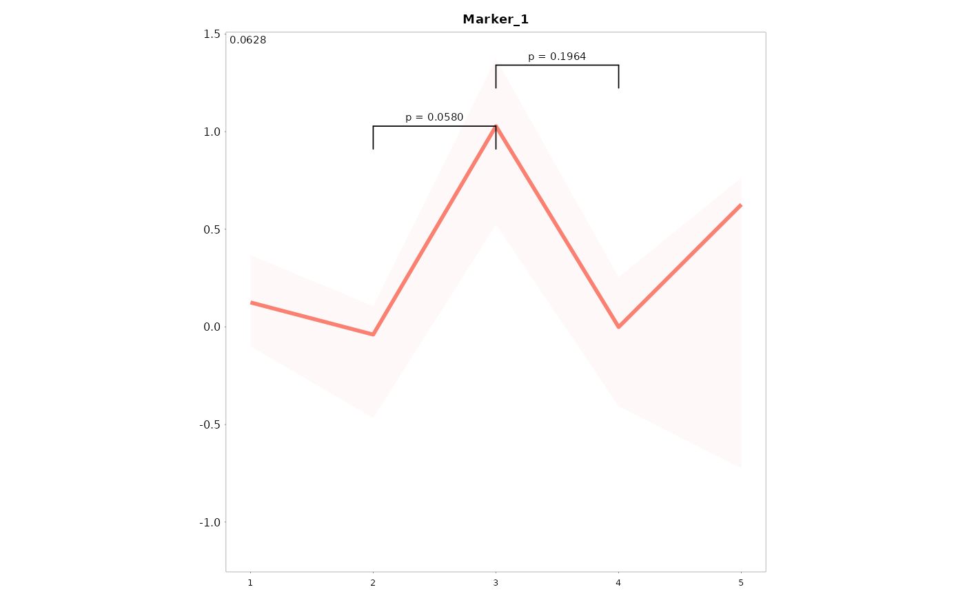
Lineplots_LB(data = data01, time = "Time", variables = "Marker_1", Overall = TRUE, Test_results = Tests[[3]], 
             Posthoc = TRUE, posthoc_test_size = 2, threshold_posthoc = 1)
#> ██████████████████████████████████████████████████████████████████████████████████████████ 100%  00:00:00 | ETA: 00:00:00 | RAM: 0.10Gb
#> [[1]]